Last modified: February 26, 2007
This thread uses PINTofALE to generate a simulated Chandra High-Energy Transmission Grating Spectrometer (HETGS) spectrum, and in particular, we will examine the O VII density-sensitive triplet as seen in the Medium Energy Grating (MEG). The Chandra ARF and RMF used were obtained from the Chandra Proposal Information page and are assumed to be placed in the current working directory.
#	start IDL
idl

;	set up the PoA environment
;
.run initale

;NOTE:
;	if INITALE fails, run the script
;	@PoA_constructor
; Because some variables will be used repeatedly in the course of this
; thread, it might be useful to initiate them now. Nailing down these
; variables now will also allow for something of a checklist for some
; important quantities/files needed for the task at hand:
; Source We will characterize our model source by the following:
!NH = 3e20 ; H column density [cm^-2]
EDENS1 = 1e09 ; electron number density [cm^-3]
EDENS2 = 1e12 ; electron number density [cm^-3]
!ABUND = getabund('grevesse') ; elemental abundances (SEE: getabund())
T_components = [6.3, 6.4, 7.4] ; log(T[K]) components in the EM
EM_components = [6.1, 6.1, 7.1]*1d12 ; Emission Measure [cm^-3]
; Observation The observation can be described by:
EXPTIME = 50. ; nominal exposure time [ks]
file_GRMF = 'aciss_meg1_cy09.grmf' ; full path name to grating RMF
file_ARFp = 'aciss_meg1_cy09.garf' ; full path name to +ve order grating ARF
file_ARFn = 'aciss_meg-1_cy09.garf' ; full path name to -ve order grating ARF
; Atomic Database We have '$CHIANTI','$SPEX','$APED' to choose from:
!LDBDIR = '$SPEX'
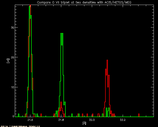
; Analysis Parameters Theoretical wavelengths for the OVII
; triplet (APED) are: 21.601(r),21.804(i), and 22.098(f), so to
; maximize our efficiency we can restrict the wavelength range:
!WMIN = 21.5 ; minimum wavelength for output spectrum [ang]
!WMAX = 22.4 ; maximum wavelength for output spectrum [ang]
nwbin = 400L ; number of bins in theoretical spectrum
;	A Differential Emission Measure (DEM) is required to estimate the
;	amount of emission at various temperatures. Typically, a 2-temperature
;	model is used. Here we will use PINTofALE's mk_dem(), which constructs
;	a DEM array given a temperature grid and emission measure components.
;	We use as the temperature grid !LOGT. The emission measure components
;	are T_components and EM_components as defined above. We choose 'delta'
;	to treat the EM components as delta functions (see mk_dem() or the
;	Chandra/ACIS example for more options)

!DEM=mk_dem('delta', logT = !LOGT, pardem=T_components, indem=EM_components)

plot,!LOGT,!DEM,xtitle='log!d10!n(T [K])',ytitle='DEM [cm!u-5!n/logK]'
;	We will assume that a ROSAT/PSPC count rate is available,
;	and that the simulation will match this rate.  We will assume
;	a count rate of 0.2 cts/s .  Data from other missions such
;	as ASCA, BeppoSAX, etc. can be dealt with in the same manner.

;	First find and read in the ROSAT/PSPC effective area.
;	You will need to know where your local PIMMS installation
;	is to do this.

pimmsdir='/soft/pimms/data'
rosat_pspc_open=get_pimms_file('ROSAT','PSPC','OPEN',pdir=pimmsdir)
rd_pimms_file, rosat_pspc_open, pspc_effar, pspc_wvlar, /wave

;	Make sure that the wavelengths are sorted in increasing order

ae=sort(pspc_wvlar) & pspc_wvlar=pspc_wvlar[ae] & pspc_effar=pspc_effar[ae]

;	The following is similar to the process described in the detailed
;	example thread (see Section 1 and Section 2).
;	For a scripted example with less details, see the companion thread
;	on the low-resolution spectrum generation.


        A] Read in line cooling emissivities and calculate line intensities

        ;Read line cooling emissivities of all possible
        ;lines in the ROSAT/PSPC wavelength range from the atomic data base.

	!EDENS=EDENS1
        lconf=rd_line(atom,n_e=!EDENS,wrange=[MIN(pspc_wvlar),MAX(pspc_wvlar)],$
	              dbdir=!LDBDIR,verbose=!VERBOSE,wvl=LWVL,logT=LLOGT,Z=Z,$
                      ion=ION,jon=JON,fstr=lstr)


        ;The output of rd_line() will only include level population,
        ;and not ion balances. We will use fold_ioneq() to fold ion balances.
        ;NOTE: This step should not be performed if !LDBDIR is set to APED,
	;which already includes ion balances and abundances.

	if strpos(strlowcase(!LDBDIR),'aped',0) lt 0 then lconf=$
	   fold_ioneq(lconf,Z,JON,chidir=!CHIDIR,$
	   logT=LLOGT,eqfile=!IONEQF,verbose=!VERBOSE)

	;NOTE: If !LDBDIR is set to APED, Anders & Grevesse abundances
	;are already included in the emissivities.  In such cases, either
	;leave out the atomic numbers (Z) in the call to LINEFLX() below,
	;or redfine the abundance array to be relative to the APED values,
	;e.g.,

        if strpos(strlowcase(!LDBDIR),'aped',0) ge 0 then $
           !ABUND = !ABUND/getabund('anders & grevesse')

	;And now calculate line intensities using lineflx().

        linint=lineflx(lconf,!LOGT,LWVL,Z,DEM=!DEM,abund=!ABUND) ;[ph/s]


        B] Read in continuum emissivities and calculate continuum intensities

        ;We can read in continuum emissivities using rd_cont().
        ;It is important to note that the output emissivities of rd_cont()
        ;are in [1e-23 erg cm^3/s/Ang] and not [1e-23 erg cm^3/s] as with rd_line()

	!EDENS=EDENS1
        cconf=rd_cont(!CEROOT,n_e=!EDENS,wrange=[min(pspc_wvlar),max(pspc_wvlar)],$
                      dbdir=!CDBDIR,abund=!ABUND,verbose=!VERBOSE,$
                      wvl=CWW,logT=ClogT)

        ;The continuum intensities per angstrom can be calculated again using
	;lineflx(). Note that CWW contains the wavelength bin boundaries for
	;the emissivity array.

        CWVL=0.5*(CWW[1:*]+CWW)
        conint=lineflx(cconf,!LOGT,CWVL,DEM=!DEM)   ;[ph/s/Ang]

        ;Now to get just continuum intensity, we must multiply by an array
	;containing the bin widths. If we define this array simply
	;with:  CDW=CWW[1:*]-CWW, we will get an ugly 'saw-toothed' figure.
	;(a side-effect of the way the data-base is constructed) To work
	;around this, we can use CWVL, the mid-bin values, and mid2bound(),
	;which gives intelligent bin-boundary values given mid-bin values:

	CWB=mid2bound(CWVL) & CDW=CWB[1:*]-CWB
	conint=conint*CDW	;[ph/s/Ang]*[Ang]


        C] Correct for inter-stellar absorption

        ;Derive ISM absorptions using ismtau()
	ltau=ismtau(LWVL,NH=!NH,fH2=!fH2,He1=!He1,HeII=!HeII,$
	            Fano=Fano,wam=wam,/bam,abund=!ABUND,verbose=!VERBOSE)
	ctau=ismtau(CWW,NH=!NH,fH2=!fH2,He1=!He1,HeII=!HeII,$
	            Fano=Fano,wam=wam,/bam,abund=!ABUND,verbose=!VERBOSE)
	ltrans=exp(-ltau) & ctrans=exp(-ctau)

        ;Derive theoretical line fluxes
	linflx = linint * ltrans	;[ph/s/cm^2]

        ;Derive theoretical continuum fluxes
	conflx = conint * ctrans	;[ph/s/cm^2]


        D] Bin spectra and fold in effective area

        ;make input theoretical spectrum grid
        dwvl=float((MAX(pspc_wvlar)-MIN(pspc_wvlar))/nwbin)
	wgrid=findgen(nwbin+1L)*dwvl+MIN(pspc_wvlar)

        ;Rebin to form theoretical line spectrum using hastrogram()
	linspc = hastogram(abs(LWVL),wgrid,wts=linflx)	;[ph/s/cm^2/bin]

        ;Rebin to form theoretical continuum spectrum using rebinw()
	conspc = rebinw(conflx,CWVL,wgrid,/perbin)	;[ph/s/cm^2/bin]

        ;Derive predicted flux spectrum.
	WVLS=0.5*(WGRID[1:*]+WGRID)
	newEffAr=(interpol(pspc_effar,pspc_wvlar,WVLS) > 0) < (max(pspc_effar))
	flxspc = (linspc + conspc) * newEffAr

        ;Derive predicted counts spectrum.
	flxspc=flxspc*EXPTIME*1e3		;[ct/bin]


;	Now get the total count rate and renormalize the DEM to the
;	observed rate of 1.0 ct/s.

obs_rate = 1.0                             ;[ct/s]
pred_rate = total(flxspc/EXPTIME/1e3)       ;[ct/s]
print,'normalization factor: ',obs_rate/pred_rate
;normalization factor:      0.024352574
!DEM = !DEM * obs_rate/pred_rate
;	The construction of the simulated spectra is largely a
;	repetition of the steps carried out to rescale the DEM.
;	It is in fact different only in three aspects: we will use
;	Chandra's instrumental response files and account for
;	differences in plus/minus orders.  Also, we will convolve
;	the resulting spectrum with an RMF (for the DEM normalization,
;	only the total counts was important). Thridly, because we
;	seek to look at the Oxygen triplet, we can concentrate on
;	a small wavelength range, and will read from the emissivity
;	databases accordingly.  We will repeat steps A through D as
;	above, and add a step E, RMF Convolution.  Also, we will
;	simultaneously construct spectra at two different densities:
;		ne = 1012 and 109 [cm-3]


        A] Read in line cooling emissivities and calculate line intensities

	;first at the higher density

	!EDENS=EDENS2
	lconf_12dex=rd_line(atom,n_e=!EDENS,wrange=[MIN(pspc_wvlar),MAX(pspc_wvlar)],$
			dbdir=!LDBDIR,verbose=!VERBOSE,wvl=LWVL,logT=LLOGT,Z=Z,$
			ion=ION,jon=JON,fstr=lstr)
        if strpos(strlowcase(!LDBDIR),'aped',0) lt 0 then lconf_12dex=$
	   fold_ioneq(lconf_12dex,Z,JON,chidir=!CHIDIR,logT=LLOGT,$
			eqfile=!IONEQF,verbose=!VERBOSE)
        linint_12dex=lineflx(lconf_12dex,!LOGT,LWVL,Z,DEM=!DEM,abund=!ABUND) ;[ph/s]

        ;now at the lower density

	!EDENS=EDENS1
	lconf_09dex=rd_line(atom,n_e=!EDENS,wrange=[MIN(pspc_wvlar),MAX(pspc_wvlar)],$
			dbdir=!LDBDIR,verbose=!VERBOSE,wvl=LWVL,logT=LLOGT,Z=Z,$
			ion=ION,jon=JON,fstr=lstr)
         if strpos(strlowcase(!LDBDIR),'aped',0) lt 0 then lconf_09dex=$
           fold_ioneq(lconf_09dex,Z,JON,chidir=!CHIDIR,logT=LLOGT,$
			eqfile=!IONEQF,verbose=!VERBOSE)
        linint_09dex=lineflx(lconf_09dex,!LOGT,LWVL,Z,DEM=!DEM,abund=!ABUND) ;[ph/s]


        B] Read in continuum emissivities and calculate continuum intensities

	;at the higher density

	!EDENS=EDENS2
        cconf_12dex=rd_cont(!CEROOT,n_e=!EDENS,wrange=[!WMIN,!WMAX],$
			dbdir=!CDBDIR,abund=!ABUND,verbose=!VERBOSE,$
			wvl=CWW,logT=ClogT)
        CWVL=0.5*(CWW[1:*]+CWW)
        conint_12dex=lineflx(cconf_12dex,!LOGT,CWVL,DEM=!DEM)       ;[ph/s/Ang]
        CWB=mid2bound(CWVL) & CDW=CWB[1:*]-CWB
        conint_12dex=conint*CDW	;[ph/s/Ang]*[Ang]

        ;at the lower density

	!EDENS=EDENS1
        cconf_09dex=rd_cont(!CEROOT,n_e=!EDENS,wrange=[!WMIN,!WMAX],$
			dbdir=!CDBDIR,abund=!ABUND,verbose=!VERBOSE,$
			wvl=CWW,logT=ClogT)
        CWVL=0.5*(CWW[1:*]+CWW)
        conint_09dex=lineflx(cconf_09dex,!LOGT,CWVL,DEM=!DEM)       ;[ph/s/Ang]
        CWB=mid2bound(CWVL) & CDW=CWB[1:*]-CWB
        conint_09dex=conint*CDW	;[ph/s/Ang]*[Ang]

	;NOTE: there is expected to be no difference between the above two
	;because continuum emissivities are density independent for the
	;parameter space we are operating in


        C] Correct for inter-stellar absorption

	ltau=ismtau(LWVL,NH=!NH,fH2=!fH2,He1=!He1,HeII=!HeII,$
	            Fano=Fano,wam=wam,/bam,abund=!ABUND,verbose=!VERBOSE)
	ctau=ismtau(CWW,NH=!NH,fH2=!fH2,He1=!He1,HeII=!HeII,$
	            Fano=Fano,wam=wam,/bam,abund=!ABUND,verbose=!VERBOSE)
	ltrans=exp(-ltau) & ctrans=exp(-ctau)

	linflx_12dex = linint_12dex * ltrans	                ;[ph/s/cm^2]
	conflx_12dex = conint_12dex * ctrans	                ;[ph/s/cm^2]
	linflx_09dex = linint_09dex * ltrans	                ;[ph/s/cm^2]
	conflx_09dex = conint_09dex * ctrans	                ;[ph/s/cm^2]


	D] Bin spectra and fold in effective area

        dwvl=float((!WMAX-!WMIN)/nwbin) & wgrid=findgen(nwbin+1L)*dwvl+!WMIN
        linspc_12dex = hastogram(abs(LWVL),wgrid,wts=linflx_12dex) ;[ph/s/cm^2/bin]
	conspc_12dex = rebinw(conflx_12dex,CWVL,wgrid,/perbin)     ;[ph/s/cm^2/bin]
        linspc_09dex = hastogram(abs(LWVL),wgrid,wts=linflx_09dex) ;[ph/s/cm^2/bin]
	conspc_09dex = rebinw(conflx_09dex,CWVL,wgrid,/perbin)     ;[ph/s/cm^2/bin]

        ;Read in the effective areas using rdarf()

        effar_p=rdarf(file_ARFp,ARSTRp)
	effar_n=rdarf(file_ARFn,ARSTRn)
	wvlar_p=!fundae.KEVANG/(0.5*(ARSTRp.ELO+ARSTRp.EHI))
	wvlar_n=!fundae.KEVANG/(0.5*(ARSTRn.ELO+ARSTRn.EHI))

	WVLS=0.5*(WGRID[1:*]+WGRID)
	newEffArP=(interpol(EFFAR_p,WVLAR_p,WVLS) > 0) < (max(EFFAR_p))
	newEffArN=(interpol(EFFAR_N,WVLAR_n,WVLS) > 0) < (max(EFFAR_n))

        ;[ct/s/bin] (if DEM is [cm-5]: [ct/s/cm2/bin])
	flxspcP_12dex = (linspc_12dex + conspc_12dex) * newEffArP
	flxspcN_12dex = (linspc_12dex + conspc_12dex) * newEffArN
	flxspcP_09dex = (linspc_09dex + conspc_09dex) * newEffArP
	flxspcN_09dex = (linspc_09dex + conspc_09dex) * newEffArN

        ;Derive predicted counts spectrum for +1 -1 orders
	flxspcP_12dex=flxspcP_12dex*EXPTIME*1e3		         ;[ct/bin]
	flxspcN_12dex=flxspcN_12dex*EXPTIME*1e3		         ;[ct/bin]
	flxspcP_09dex=flxspcP_09dex*EXPTIME*1e3		         ;[ct/bin]
	flxspcN_09dex=flxspcN_09dex*EXPTIME*1e3		         ;[ct/bin]
	EGRID=!fundae.KEVANG/WGRID


	E] Convolve with RMF

	conv_rmf,EGRID,flxspcP_12dex,CHANP,CTSPCP_12dex,file_gRMF,rmfstr=grmf
	conv_rmf,EGRID,flxspcN_12dex,CHANN,CTSPCN_12dex,grmf
	conv_rmf,EGRID,flxspcP_09dex,CHANP,CTSPCP_09dex,grmf
	conv_rmf,EGRID,flxspcN_09dex,CHANN,CTSPCN_09dex,grmf


;	Combine the two output spectra to get a co-added first order spectrum.

CHAN_dens_12dex=CHANP                            ;[keV]
cts_dens_12dex=ctspcP_12dex+ctspcN_12dex         ;[ct/bin]
CHAN_dens_09dex=CHANP                            ;[keV]
cts_dens_09dex=ctspcP_09dex+ctspcN_09dex         ;[ct/bin]

;	We thus obtain co-added spectra at two densities.

;	Note that the output energy grid of the spectra will be by
;	default the energy grid defined by the RMF.  The spectrum
;	however will only show lines and continuum between the
;	selected wavelength ranges.
;	The final step is a simulation of counts based on the spectrum
;	predicted above

nbin = n_elements(cts_dens_12dex)
CTSIM_dens_12dex=intarr(nbin) & CTSIM_dens_09dex=intarr(nbin)
for i=0L,nbin-1L do if cts_dens_12dex[i] gt 0 then $
    CTSIM_dens_12dex[i]=randomu(seed,poisson=cts_dens_12dex[i])
for i=0L,nbin-1L do if cts_dens_09dex[i] gt 0 then $
    CTSIM_dens_09dex[i]=randomu(seed,poisson=cts_dens_09dex[i])

;	Now to make a comparison plot of the OVII triplet at
;	two densities (red: ne=1012 cm-3; green: ne=109 cm-3):

plot, !fundae.KEVANG/CHAN_dens_12dex, CTSIM_dens_12dex, /nodata,$
	title='Compare O VII triplet at two densities with ACIS-S+HETGS/MEG',$
	xtitle='['+!AA+']', ytitle='[ct]', ystyle=1, xstyle=1,$
	xrange=[!WMIN,!WMAX], yrange=[0,1.1*max(CTSIM_dens_12dex)], thick=2, psym=10
oplot, !fundae.KEVANG/CHAN_dens_12dex, CTSIM_dens_12dex, color=2, psym=10, thick=2
oplot, !fundae.KEVANG/CHAN_dens_09dex, CTSIM_dens_09dex, color=3, psym=10, thick=2
stample
(Images generated with AO-7 RMF and ARF files)